How a 1820 discovery maps the invisible magnetic fields surrounding every electric current
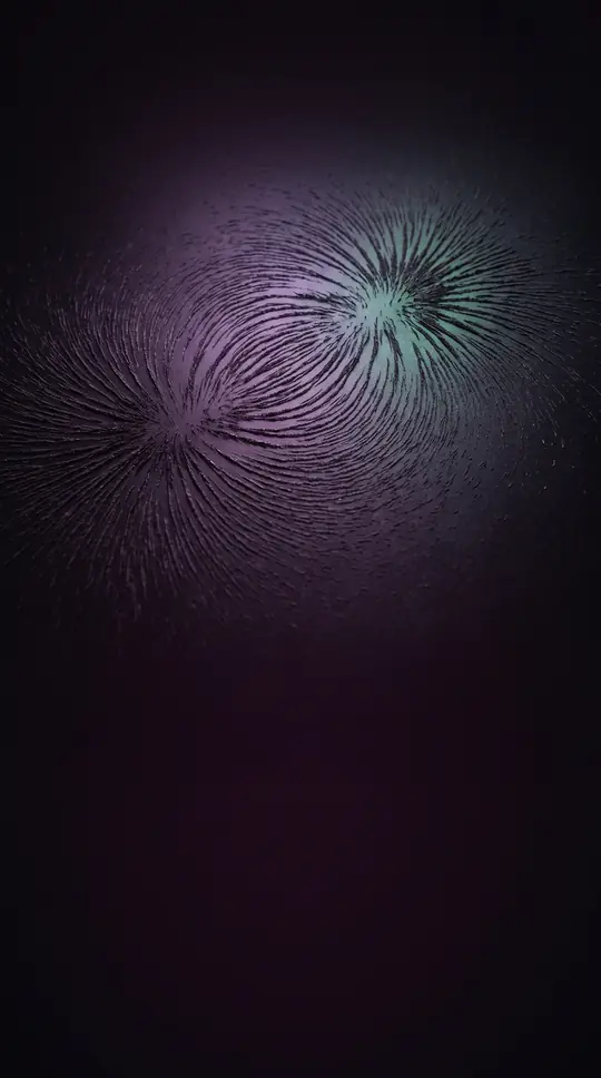
In short: In 1820, Jean-Baptiste Biot and Félix Savart uncovered a fundamental relationship between electric currents and the magnetic fields they generate. This law remains a cornerstone of magnetostatics, allowing physicists to calculate the magnetic influence of everything from simple wires to complex solar flux ropes and quantum vortex filaments.
The Biot–Savart law provides a quantitative method to determine the magnetic field generated by a steady electric current. At its core, the law describes the magnetic field as a vector sum, relying on the superposition principle: the total magnetic field at any point is the result of summing the individual contributions from every infinitesimal segment of the current-carrying conductor. For a small segment of wire, the magnetic field contribution is proportional to the current and inversely proportional to the square of the distance from the segment to the observation point.
While the law is mathematically elegant, applying it to real-world scenarios often requires significant computational power. For simple, infinitely long wires, the field can be expressed through a straightforward formula, but more complex geometries—such as loops, solenoids, or the curved axes of solar flux ropes—require evaluating line integrals. In cases where conductors have thickness, the law is reformulated to account for current density throughout a volume, rather than just along a filamentary path. These calculations are essential in fields ranging from astrophysics, where they help model coronal mass ejections, to quantum physics, where they simulate turbulence in superfluid helium.
It is important to distinguish the true Biot–Savart law from related approximations. For instance, some equations describing moving point charges are occasionally mislabeled as Biot–Savart laws due to their superficial resemblance, even though the original law strictly applies to steady, stationary currents. Furthermore, researchers must be cautious with simplifications like the localized induction approximation (LIA). While LIA can simplify calculations, it often fails to capture the full physical reality of complex systems like quantum turbulence, where the full Biot–Savart integral is necessary to achieve accurate, statistically steady results.
Opens the Intellect+ feed with this card first. Swipe up for the next one.
Sources
- Summary by Intellect · source: Biot-Savart law | Definition, Formula, Diagrams, & Facts | Britannica
- Also: Biot–Savart law
- Also: Steady-state counterflow quantum turbulence: Simulation of vortex filaments using the full Biot-Savart law
- Also: Regularized Biot–Savart Laws for Modeling Magnetic Flux Ropes
To cite this card, link to https://intellectplus.co.uk/app/science-biot-savart-law.
How we source, check and correct cards: Editorial standards.
General information, not professional advice. Spotted an error? Flag the card or see corrections and complaints.
Intellect Plus is a visual educational discovery platform for exploring fascinating facts and ideas. Brain Food, Not Brain Rot. What is Intellect Plus?
Related
More in Physics · More in Science · Latest · A–Z · All topics
